Poynting-Robertson effect
The Poynting-Robertson effect consists of the Poynting-Robertson drag and the radiation pressure force. The Poynting-Robertson effect is implemented according to [BurnsLamySoter79] and is available in the schemes (we recommend scheme 1):
The following parameters are relevant for the Poynting-Robertson effect and can be set in the param.dat file:
Use Poynting-RobertsonSolar Constant: Solar Constant at 1 AU in W /m^2Radiation Pressure Coefficient Qpr(in general assumed to be 1)
Solar Wind
Solar wind drag can be added to the Poynting-Robertson effect according to [LZJ95]. The solar wind drag is only applied in scheme 1. Enable it with:
Solar Wind factor, only applied to scheme 1.
Scheme 1: Velocity kick
The Poynting-Robertson effect is implemented according to the following equation:
When solar wind is included, then the following equation is used:
where \(sw\) is the ratio of solar wind drag to Poynting-Robertson drag.
Scheme 2: orbital averaged drift rates
Set the call interval
With the parameter Poynting-Robertson Inteval the calling interval of the Poynting-Robertson function can be set. This means that
the function is called fewer times, and in increased drift rate \(dx = a * dt * Poynting-RobertsonInterval\).
With the time averaged Poynting-Robertson function (mode 2) it is possible to use quite large interval numbers.
The direct Yarkovsky effect (mode 1) is more sensitive to values greater than \(\approx 100\).
Strictly speaking ,this argument violets the symplectic nature of the integrator, but as long as the Yarkovky force is small it is OK.
Test of the Poynting-Robertson effect
In Fig. 14 is shown a test of the Poynting-Robertson effect for the same initial conditions as in Test of the Yarkovsky effet, but with eccentricities \(\neq\) 0.
Use Poynting-Robertson = 1 (2)
Solar Constant = 1367
Radiation Pressure Coefficient Qpr = 1
Semi-major axis a = 2 AU
Eccentricity = 0.05
Inclination = 0
Argument of perihelion = 0 - 2 \(\pi\)
Longitude of ascending node = 0 - 2 \(\pi\)
Mean anomaly = 0 - 2 \(\pi\)
Density \(\rho\) = 3500.0 kg/m^3
Physical radius R = 0.1 - 100 m
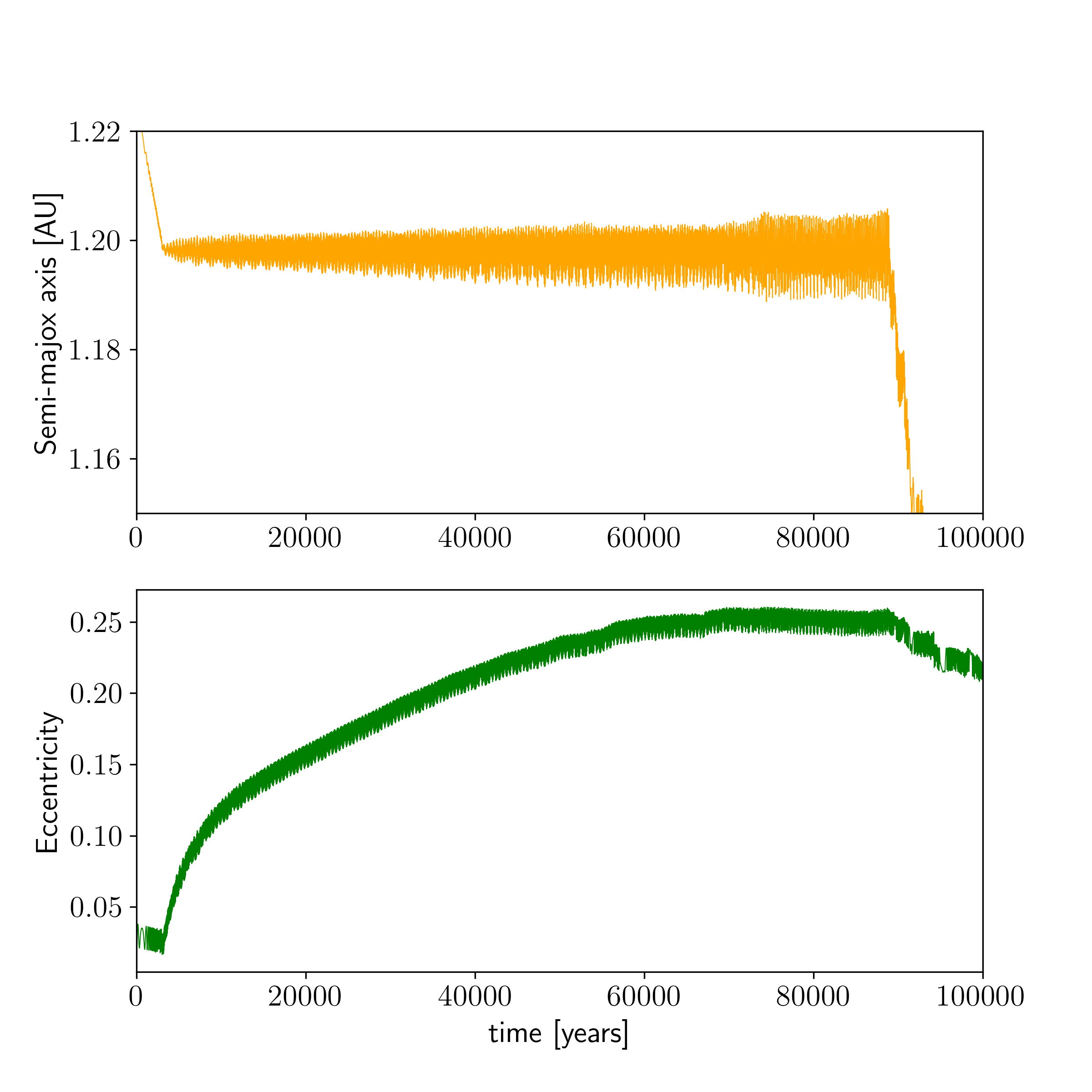
Fig. 14 Drift rate of the Poynting-Robertson effect. Computed after 10000 years and averaged over 1 orbit.